Preparation
View Lloyd Rieber's pre-recorded presentation of an instruction to quantitative research methods, corresponding to chapters 8-11 of the 10th edition of the Leedy and Ormrod textbook. This can be found on your course learning plan.
Directions
In this activity, you will compute the t statistic using the data set used in the previous activity as the pretest plus a set of posttest scores that will be emailed to you. You will use the Excel spreadsheet file that you created in the previous activity. Save this updated Excel file as "yourLastName-statistics2.xls" (e.g. Jones-statistics2.xls).
Lloyd Rieber has prepared a video tutorial for you. Follow the video instructions carefully as you work with Excel. When finished, email your Excel file as an attachment to Lloyd Rieber at lrieber@uga.edu with the subject line: "yourLastName - Statistics Activity 2."
The video is approximately 18 minutes in length. Click on the following link to launch the video in a new window:
- Computing a t statistic (17:02)
I hope you will enjoy this activity and find it relevant and satisfying.
Resources
You will use two formulas in this activity. Consult these formulas often as you complete the activity.
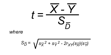
The first is the standard formula for computing the t test:
However, as you can see, computing the standard error of the difference (i.e. "S sub d bar") between the correlated means is rather daunting. Fortunately, there is an easier way to do the computation. But, before we explore this easier way, notice that this term uses r, which is a correlation coefficient. That is important because it shows that this statistic is based on computing a correlation between the two means.
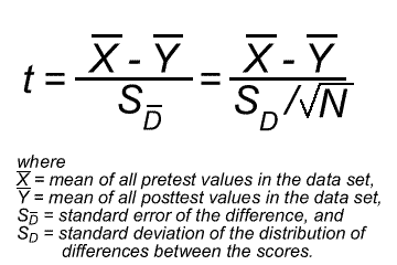
OK, here is a second version of the t test that is much easier to compute:
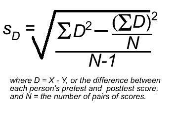
And, here is the formula for computing the standard deviation of the distribution of differences between the scores:
As you can see, this formula uses the sums of the differences between each person's pretest and posttest score. Doing this is a snap in Excel.
Determining if you should reject the null hypothesis based on the t value
After you compute the t statistic, you will need to determine whether the difference between the means is statistically significant based on a predetermined probability (usually .05, meaning 95 times out of a 100, the differences would not be due to chance). Traditionally, to do this, one would look up the value on a t distribution table. But, here is a nice web site that will compute the probability value for you:
t test calculator (danielsoper.com)
You will need to enter your t value along with the degrees of freedom (df) of your sample. For a correlated t test, the degrees of freedom is always N-1 (number of participants minus one).
If the probability value shown by the calculator for a two-tailed test is less than .05, you should "reject the null hypothesis" (recall that the null hypothesis is that both means are equal) and conclude that the means are, in fact, significantly different from one another. One could then say with confidence that the instructional intervention made the difference in having the posttest scores increase from the pretest scores.
Finally, it is important to note that t tests, like most inferential statistics, are only robust if all the assumptions on which they are based are met. For example, an important assumption is that there is a large enough N, or number of participants in the sample. As a rule of thumb, the smallest N should be around 30, but the larger the better.


